
EBSD Explained
Techniques
Applications
Hints and Tips
Technology
OXFORD INSTRUMENTS EBSD PRODUCTS
CMOS Detector RangeAZtecHKL Acquisition SoftwareAZtecCrystal Processing Software
The data collected with Electron Backscatter Diffraction (EBSD) contain a wealth of sample information which can be processed using a suite of analytical tools to visualise and represent microstructure at the micro and nano scale. Unlike many associated electron microscopy techniques, such as energy dispersive X-ray spectrometry (EDS), EBSD analyses typically involve a significant time processing and interrogating the datasets away from the microscope.
The spatially-linked crystallographic orientation and phase information acquired with EBSD can be processed to deliver information about the sample, which in turn can be linked to the materials processing history and physical properties. Typical measurements can include:
In the tabs below we look at 4 main categories of EBSD data representation, namely grain size, texture, boundaries and maps, giving examples of how these can be used to highlight and understand aspects of a sample’s microstructure.
A grain can be considered as a three-dimensional crystalline volume within a specimen that differs in crystallographic orientation from its surroundings but, internally, has little orientation variation. Grain size is an important characteristic used in understanding the development, engineering and potential failure in materials, not least because the mechanical and physical properties of metallic materials are often related to their grain size (e.g. via the Hall-Petch relationship where strength is inversely dependent on the square root of grain size). EBSD is an ideal technique for determining this grain size, as it combines exceptional spatial resolution and the capability to analyse large areas (and hence many 1000s of grains) very quickly with a quantitative rigour that is missing from other techniques.
To accurately measure grain size, it is imperative that all of the grain boundaries are firstly defined and then reliably detected. Traditionally grain size was measured using light optical microscopy (LOM) and some of the grain size standards still reference this method. This optical technique usually requires a chemical etching of the surface in order to highlight the grain boundaries. However, this etching can be influenced by the existing microstructure in the sample, which can be problem for fine structured materials. In addition, as the trend is towards nano scale materials, there is a limit to the grain size which can be detected by LOM (as governed by the wavelength of visible light).
Therefore, EBSD has become the most attractive, viable alternative for measuring grain size, even without considering the vast amount of additional microstructural information that the technique can provide.
To identify the grains using EBSD requires the definition of a critical disorientation angle, so that all boundary segments with an angle higher than this defined critical angle are considered grain boundaries. Note the use of “disorientation”, as this is the accepted term to denote the smallest of all the crystallographically-equivalent misorientation angles which, by convention, is the angle that we use. By measuring the disorientation between all adjacent pixel pairs, it is possible to identify the boundaries enclosing the individual grains. However, in many materials there are special boundaries (such as twin boundaries) that we do not want to consider as grain boundaries. These can be rigorously defined in EBSD datasets, using the crystallographic relationship between adjacent twin domains and then they can be effectively excluded from the grain measurement.
There exist several international standards that provide guidance on the correct methodology for measuring grain sizes using EBSD. The most important parameters for 3 of these standards are summarised in the table below.
| GB/T 35165-2018 | ISO 13067:2011 | ASTM E2627 - 2013 | |
| Data Clean up | Total hit rate increasing < 5% | Total hit rate increasing < 5% | Total hit rate increasing < 10% |
| Minimum Grain Boundary Disorientation | 5°~15° | >=5° for equiaxed grain structures Larger angles for other materials, typically 10° or 15° | 5° |
| Number of pixels per grain | ≥10 | ≥10 | ≥100 |
| Number of scan fields | ≥3 fields, each ≥50 grains | ≥3 fields, each ≥50 grains | At least 50 grains in any scan field |
| Total number of grains | ≥500 | ≥500 - 1000 | ≥500 |
Table comparing some of the critical parameters for measuring grain size using EBSD, for different international standards.
Regardless of which standard (if any) is to be followed, the most important aspect of any grain size measurement is that all the measurement criteria are reported along with the grain size data.
Once the grain boundaries have been detected, for every phase in the sample each grain can be measured to provide all the standard grain size and morphological information. In addition, orientation data from each pixel can be used to characterise the internal crystallographic properties of the grains (such as the degree of lattice orientation variation, as shown in the example on the right).

Grain Orientation Spread (GOS) map of a shot peened aluminium in cross section. This valuable primary strain analysis tool reveals grains that show the most deformation - it illustrates their spatial distribution and numerical prevalence. It is a whole grain classification tool: for each grain in the mapped area, GOS measures the degree of orientation change between every pixel in the grain and the grain’s average orientation. The grain is then coloured by the average measurement for all of its constituent pixels. Grains with a higher level of strain, measured by the internal degree of lattice rotation, are coloured at the yellow - red end of the rainbow colour scale shown in the histogram. In this example, the grains exhibiting higher levels of strain are concentrated near the surface, within a damage zone extending to approximately 150 μm below the surface.
Having followed the necessary procedure for measuring the grain size using EBSD data, there are multiple ways to represent the data in the form of maps, histograms or statistics. EBSD software will usually enable all of these approaches, but typically the output will depend on the application and the information that is required.
Grain statistics, relating to entire data set or restricted to selected phases, are generated from the grain measurement and can provide the necessary information to characterise the sample’s grain size. However, as shown by the example from the shot-peened Al sample shown earlier, the grain data can be used to examine particular aspects of the microstructure, such as the extent of plastic deformation or the area fraction of recrystallisation, or can be used to sub-divide the data into individual subsets that can then be examined separately (e.g. large grains v small grains).
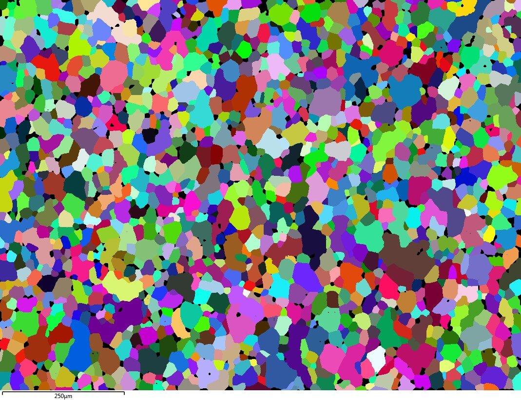
EBSD grain map from a single phase steel sample, showing grains in random colours. Grains were detected using a grain detection angle of 10° and a minimum 100 pixels within a grain (as recommended by the ASTM E2627 standard). 1378 grains are detected with a mean grain diameter of 25.5 μm.

EBSD grain data from the same steel sample shown above. The full grain details and statistics are summarised, using EBSD processing software.
Perhaps the most common approach is to plot maps showing the grain size (e.g. using the grain area or an equivalent circle diameter), plus a grain size histogram. This is shown in the example below, from a dataset taken from a rolled duplex stainless steel. However, it is important to note that the histogram does not represent the grain size distribution but is the distribution of 2D size only and will be very strongly affected by the sectioning effect.


Grain data from a rolled duplex stainless steel. Left – Grain size map (using the equivalent circle diameter - ECD). Right – grain size histogram for the austenite phase (Fe-FCC), along with corresponding statistics. Note that Sigma 3 twin boundaries were excluded from the grain size measurement.
A training video on how to measure grain size from EBSD data using AZtecCrystal can be viewed in the Training Hub section of the website, here.
Representing texture (or crystallographic / lattice preferred orientation) as measured by EBSD can be a challenge: effectively you need to represent 3D orientation data using a 2D medium. This is primarily achieved using either pole figures, inverse pole figures or orientation distribution functions (ODFs), but useful texture information can also be plotted in maps.
Pole figures are perhaps the most common way to display texture. They enable 3D orientation data to be plotted in 2D by converting crystallographic directions into points.
A pole figure is the stereographic projection of the poles (or directions) used to define the 3D orientation of the crystal lattice in the sample. The following figure gives a very basic introduction into how a pole figure is created from a cubic unit cell.
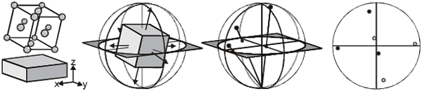
Illustration showing how a 3D orientation is displayed in a pole figure (for a cubic crystal). Note the solid circles in the final pole figure represent the upper hemisphere projection, the open circles the lower hemisphere projection.
Pole figures are plotted automatically with modern EBSD systems; it is usual to plot the normal (or “pole”) to a lattice plane, although sometimes it is useful to plot crystallographic directions instead. In materials science applications, the upper hemisphere projection is more common, whereas in the geological sciences a lower hemisphere projection is preferred. It is worth noting that more than 1 pole figure is required in order to show the complete 3D orientation of a crystal. For different crystal systems there are standard combinations of crystallographic poles or directions that are plotted – such as the {100}, {110} and {111} poles for cubic phases, as shown in the example below.
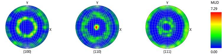
Density contoured pole figures of the β brass phase in a leaded brass sample. The clustering of the data in the central {110} pole figure indicates a strong <110> fibre parallel to Z direction.
Inverse pole figures (IPFs), as the name implies, are effectively the inverse of standard pole figures. Instead of plotting crystallographic directions in the sample reference frame, IPFs plot a sample direction in the crystallographic reference frame.
For example, an IPF plot for the rolling direction (RD) of a rolled metal sheet will plot, for each orientation measurement, the crystal direction that is parallel to the RD. This means that, instead of plotting in the full stereographical space, we plot instead in the primitive space for each crystal system. Similar to a conventional pole figure, a single IPF is not sufficient to fully define a crystal orientation, so it is convention to plot IPFs for all the 3 orthogonal sample axes (such as rolling direction, transverse direction and normal direction). An example from a rolled duplex stainless steel is shown below.

Inverse Pole Figures for the 3 orthogonal sample directions (RD, ND and TD) in a rolled sheet of duplex stainless steel, for the FCC phase. Colours correspond to the densities, indicating a strong alignment of the <101> direction with the ND, and a weaker alignment of the <001> directions with the RD.
One advantage of IPFs compared to pole figures is that, for each measurement, only a single point is plotted in each IPF.
Orientation Distribution Functions (ODFs) are a means of representing preferred orientations for materials. It is a four-dimensional object – the four dimensions being the three Euler angles and a density value corresponding to the strength of the contribution of a specific orientation. This strength is expressed as a ratio to that expected for a completely random distribution of orientations. In effect, the ODF can be defined as the volume fraction of grains with a particular orientation.
The ODF approach to texture measurements has many strengths, but also a few weaknesses (the most significant being that there is no intuitive connection between Euler space and specimen (i.e. physical) space). Traditionally most texture measurements were carried out using X-ray or neutron diffraction techniques; therefore, there exists a significant body of experimental texture data, much of it in the form of ODFs, that has been used to define many commonly found textures. However, X-ray measurements usually measure the distribution of poles and are as such incomplete, whereas EBSD texture measurements are complete and have the added advantage of being directly relatable to the microstructure. Nowadays texture measurements using ODFs derived from EBSD measurements have become widely accepted, and have largely replaced texture analyses using X-ray diffraction.
One common way to calculate ODFs is to use a “Series Expansion Method” – this 2 step approach firstly calculates the texture coefficients and then uses those coefficients to derive the actual ODF. The resulting ODF densities can then be plotted in 3-D Euler space, but more commonly sections through that space are selected (keeping one Euler angle constant) and either a series of spaced 2D sections are shown, or a specific section is chosen. For some common textures, it can be sufficient to display a density profile with 2 fixed Euler angles. An example from a rolled steel sample is shown below.


ODF Texture plots for Fe-BCC in a rolled duplex steel. Left – single section (φ2 = 45°) through the ODF Euler space showing the development of a {001}<110> texture (densities in the top corners) and an α-fibre texture (densities down the left edge). Right – density profile along the α-fibre (i.e. down the left edge of the section)
Although ODFs may not be intuitive to understand, they do permit a rigorous assessment and comparison of textures as measured by EBSD and are still the preferred approach to texture representation in a number of metals-processing industries.
As mentioned previously, EBSD has a significant advantage over other texture measurement techniques in that the textures can be related directly back to the microstructure. In other words, it is possible to observe local texture variations within a sample and to relate these to other aspects of the microstructure (such as phase distribution, strain or grain size).
Standard orientation maps (as discussed in the next tab) do highlight textures, but it is also possible to plot specific texture component maps. These show the measurement points that have an orientation within a pre-defined deviation threshold from a certain texture, and can highlight the local texture variations very effectively.
In the example below, maps have been plotted from the same leaded brass sample that was shown in the pole figures section above, highlighting the strength of the texture in the β-brass phase.


Texture analysis of a leaded brass sample. Left – phase map; red – lead, yellow - α-brass, blue - β-brass. Centre – map showing the strength of the <110> || Z direction texture in the β-brass. Right – colour key for the β-brass texture showing the deviation from the ideal <110>|| texture.
Maps are the most common way to represent EBSD data. The technique, with the rapid automated collection of orientation and phase data from a grid of points on the surface of a sample, lends itself to the display of data in map form.
There are too many map types to be addressed here, and we have already introduced grain-based maps and texture component maps in the other tabs on this page. However, there are some common map types which should almost always be used as a starting point for any EBSD analysis and these are described below.
The EBSD pattern quality parameter assigns a number to the degree of sharpness, contrast or band definition in the EBSP. Different commercial systems will utilise slightly different pattern quality parameters (sometimes referring to them as “image quality” or “IQ”), but they are all influenced by several factors: phase, orientation, contamination, sample preparation and the local crystalline perfection.
Pattern quality maps will often reveal features invisible in the electron image such as grains, grain boundaries, internal grain structure and surface damage such as scratches. Even if the EBSD indexing process is poorly set up or cannot determine reliable solutions, the pattern quality map will still show the main features of the microstructure, as shown in the example to the right. The pattern quality map is therefore very useful both during the analysis of the data and as a simple tool for checking the sample before, during and after analysis.

A pattern quality map for a Titanium (Ti6Al4V) sample. Dark areas are indicative of poorer pattern quality and light areas of higher pattern quality.
In some cases, such as in martensitic or bainitic steels, the pattern quality map contains information that can be used to separate and to classify phases. This is addressed in more detail here.

The identification and distribution of different phases is another important application of EBSD. Phases can be represented on a map, highlighting their distribution and providing accurate area fractions for each phase. A phase map is a powerful tool for numerous applications of EBSD, such as for determining the importance of precipitate formation at grain boundaries.
An example EBSD phase map of a duplex steel sample. The microstructure contains austenite (blue) and ferrite (red) phases; as well as intermetallic sigma (green) and chi (yellow) phases. These intermetallics are significant as they will degrade mechanical and corrosion properties of the material. Therefore, it is important to identify them, determine their distribution and phase fraction (as provided in the map legend).
The orientation data collected with an EBSD system is most commonly displayed in either an Euler Map or a series of inverse pole figure (IPF) maps. The Euler maps give a basic presentation of microstructure but, by the nature of the Euler measurement scheme, can be hard to interpret. The IPF maps use the colour from the IPF colour key, in this case the colour assigned is based on the measured orientation and the selected viewing direction. An IPF map is good at representing preferred orientation (texture), seen as similar or single colours in the map. The orientation data displayed in a map make it easy to visualise and extract information about how a specific texture is spatially distributed.
This is shown in the example on the right, from a sheared quartz rock. The large red area to the top left indicates the presence of a single large grain, whereas the finer grained region can be seen to contain 2 different preferred orientations, one with a green/blue dominant colour and one mostly in red. The orientation map provides an instantaneous illustration of the overall texture within the sample.

EBSD orientation map from a deformed quartz rock, showing at each point which crystal direction is parallel to the sample X direction (an “IPF-X” map), as shown in the legend.
It is important to note that one single orientation map using an IPF colouring scheme is not sufficient to fully determine the texture at each point. More details about how to interpret orientation maps can be viewed in a training video available in the Training Hub section of the website, here.
The boundaries in a material play a critical role in controlling the overall physical properties, and EBSD is an ideal technique as it provides information about 4 of the 5 parameters that are required to characterise a boundary (disorientation angle, rotation axis (2 parameters), boundary plane (2 parameters, only 1 measured by 2D EBSD).
For example, in grain boundary engineering it can be important to enhance or reduce the relative abundance of certain grain boundary types in order to optimise the properties of the final material, whereas in deformed materials the boundary disorientation angles can point to the activation of certain deformation mechanisms. EBSD is well suited to extract all the necessary information as it gives crystallographic, statistical and spatial information about the grain boundaries.
Particular boundary types can be identified through a disorientation frequency distribution histogram. Here the plot will have a distinct peak if there are many grain boundaries with a similar disorientation angle, such as might be expected for a twin boundary.

Disorientation angle frequency distribution from a deformed quartz rock.
This method is typically used to get a quick overview of the boundary occurrences in the sample, and an indication of the statistical significance of the distribution can be obtained by comparing the measured disorientation angles with those from randomly selected measurement pairs (this will indicate the effect of any texture) and with a theoretical random distribution (this will indicate the effect of the crystallographic symmetry of the phase). An example from a deformed quartz rock sample is shown above: the peak at low disorientation angles is caused by the prevalence of low angle boundaries due to the deformation, whereas the peak at 60° is attributable to a high frequency of Dauphiné twin boundaries.
Similarly, generating a map that shows the spatial distribution of the grain boundaries can provide additional microstructural information. A typical example, shown below, includes a map showing low angle boundaries (highlighting the substructure of individual grains) combined with high angle boundaries (defining the actual grain structure).

Grain boundary analysis of a steel sample using EBSD. The sample contains Ferrite (white) and Austenite (red) phases. The grain boundaries of the ferrite phase are superimposed on the phase map: low angle (2-10°) boundaries are in green, with high angle (>10°) boundaries in black. It illustrates the contrasting grain structure and substructure of individual grains in the ferrite.
When the disorientation angle is calculated it is also possible to calculate the disorientation axis. This means that EBSD data can be used to identify specific boundaries defined not just by a disorientation angle but by a combination of disorientation angle and disorientation axis. The most common example is the identification of twin boundaries, which are a subset of the coincident site lattice (CSL) boundaries.
CSL boundaries are special boundaries which fulfil the coincident site lattice criteria, whereby the lattices of the 2 adjacent crystallites are sharing some of the atomic lattice sites. CSLs are characterized by Σ where Σ is the reciprocal density of the coincident sites. Two examples of CSL relationships are shown below.

(a) The Σ3 boundary (twin boundary) is a 60° rotation about the [111] direction, with every 3rd atom coincident for both lattices. (b) The Σ5 boundary is a 36.9° rotation about the [100] direction.
CSL boundaries typically have a significant impact on the material properties, which means that from a materials engineering viewpoint it is important to determine both the ratio of CSL boundaries and their distribution within the material. An example from an austenitic steel sample is shown on the right.
The map background represents the pattern quality, with high and low angle boundaries and CSL boundaries superimposed. The legend shows that >50% of all high angle boundaries can be classed as Σ3 CSL boundaries.

CSL boundary map for an austenitic steel sample.
© Oxford Instruments 2026