
EBSD Explained
Techniques
Applications
Hints and Tips
Technology
OXFORD INSTRUMENTS EBSD PRODUCTS
CMOS Detector RangeAZtecHKL Acquisition SoftwareAZtecCrystal Processing Software
Conventional EBSD analyses use an image transform, such as the Hough transform, to identify the positions of the Kikuchi bands in each EBSD pattern and to compare these with a look up table of interplanar angles for each candidate phase. This process of pattern indexing, as explained here, is both fast and robust, providing excellent quality data at speeds in excess of 5000 indexed patterns per second.
However, an alternative approach to EBSD pattern indexing has been developed in recent years, utilising advances in diffraction pattern simulation and image correlation methods. This new approach, broadly termed “pattern matching”, has been introduced here and is growing in both popularity and functionality.
The initial development of pattern matching as a tool for EBSD analysis was initially driven by improvements in EBSD pattern simulation, most notably by the effective application of the dynamical theory of electron diffraction that could predict not only the position of Kikuchi bands in an EBSP, but also their intensities. This enabled the generation of simulated patterns that closely resembled their experimental counterparts, as shown in the image below and, from there, it became possible to match experimental EBSPs to the best fitting simulations.
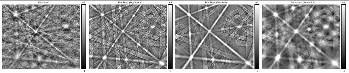
EBSD patterns from the mineral quartz (SiO2). Left to right: typical experimental EBSP, many-beam dynamical simulation, 2-beam dynamical simulation, kinematical simulation.
Key to any effective pattern matching method is a robust way to measure the degree of similarity between 2 images (e.g. an experimental and a simulated diffraction pattern). This is best done using the normalised cross correlation coefficient. The normalised cross correlation coefficient is a widely used approach in image analysis and is ideally suited for EBSD, since it can cope with significant intensity or contrast fluctuations in the images (e.g. due to different electron beam or sample conditions, or varying exposures on the EBSD detector). The basic equation is shown below, but the normalisation ensures that the mean background = 0, with the average standard deviation for each pixel = 1.
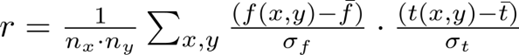
Equation for calculating the normalised cross correlation coefficient, r for a simulated template t(x,y) and an experimental pattern f(x,y), with n pixels in x and y. The average and standard deviation of f and t are denoted by f ̅ and t ̅ , and σf and σt respectively.
For EBSD pattern matching, we only consider the magnitude of r and thus see a range of values from r = 0 (indicating no correlation between the images) to r = 1 (the images are identical). In reality, due to noise in experimental patterns, the r value rarely exceeds 0.8. What value constitutes a reliable match depends very much on the quality of the patterns and the information that is being measured. For example, when indexing poor quality EBSPs (such as from highly deformed structures) a match with r > 0.15 will likely indicate a correct indexing, whereas when trying to determine crystal polarity or to resolve subtle pseudosymmetry relationships, a match with r > 0.5 will likely be required, with the best solution having an r value at least 0.01 higher than the 2nd best solution.
The pattern matching functionality implemented in AZtecCrystal MapSweeper enables all types of EBSD data enhancement, including full indexing, improvements in data quality or the extraction of new information from EBSD patterns. These tools are based on full dynamical pattern simulations (although 2-beam and kinematic simulations can be used) and they use the normalised cross correlation coefficient as the most robust metric for the similarity between patterns.
In the following tabs you can learn how the different “Sweep” modes in AztecCrystal MapSweeper work and how they can be used to improve the quality of a wide variety of EBSD datasets. The gallery provides a number of varied examples showing the application of this advanced software.
AZtecCrystal MapSweeper uses a new approach to indexing – Dynamic Template Matching (DTM). The principles of DTM are similar to those used for Dictionary Indexing, but with several key differences:
The process of DTM is graphically illustrated in the following image. Note the use of lower resolution templates and a binned (lower resolution) original EBSP during the initial indexing step, followed by a refinement at a higher EBSP / template resolution to give a more precise final solution.
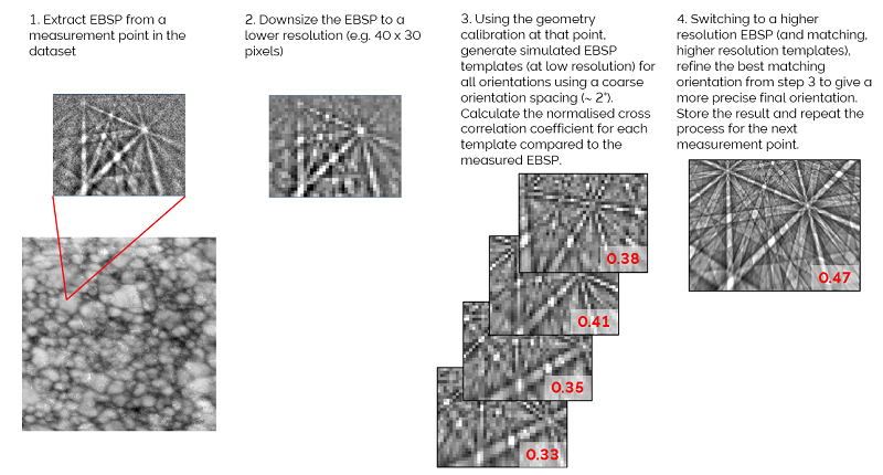
Step by step process of EBSD pattern indexing using Dynamic Template Matching (DTM). For datasets with multiple phases, this process is followed for each candidate phase and the solution with the highest normalised cross correlation coefficient is selected.
The DTM indexing method can be relatively fast, depending on the available computing power and the symmetry of the candidate phase(s). For the analysis of a single cubic phase dataset using a workstation with a mid-level GPU, typical indexing speeds will range from 25-200 patterns per second.
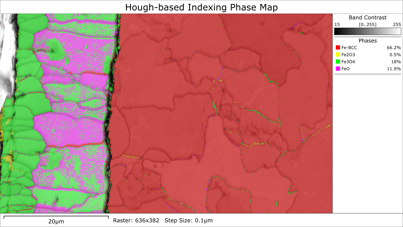
Indexing using pattern matching methods is not usually necessary – Hough-based indexing will, for most samples, provide sufficiently good data quality such that only a further enhancement is required (see the “Refine” and “Repair” tabs for more detail on so-called “Hybrid Pattern Matching” approaches). However, for some samples, such as those that produce very poor quality EBSD patterns as a result of high defect densities or nanocrystalline structures, the indexing rates using Hough-transform based methods can be unacceptably low (e.g. <50%). In such cases, a “brute force” indexing method such as DTM can be essential and will lead to significantly better data quality.
The following video illustrates how DTM indexing in AztecCrystal MapSweeper is used to analyse a nanocrystalline MgB2 superconductor. Initial Hough-based indexing resulted in only a 50% indexing rate, whereas DTM indexing achieved >90%.
Video showing the reanalysis of a challenging TKD sample using DTM indexing in AZtecCrystal MapSweeper.
The dominant utilisation of pattern matching technology within AZtecCrystal MapSweeper involves “hybrid” methods. Hybrid pattern matching is the term given to the use of pattern matching methods that involve using the pre-existing orientation and phase information, usually acquired by standard Hough-based indexing. The advantage of a hybrid method over “brute force” methods (such as Dictionary or Spherical Indexing) is that the analysis is both much faster and will typically result in significantly better-quality data. In MapSweeper, both the Refine and the Repair sweeps use Hybrid methods.
Here we describe how hybrid pattern matching is used in MapSweeper to enhance the quality of an EBSD dataset. In a Refinement Sweep, MapSweeper can improve the orientation precision, resolve pseudosymmetry, resolve crystal polarity and improve phase separation. These analytical goals are considered separately in the following sections.
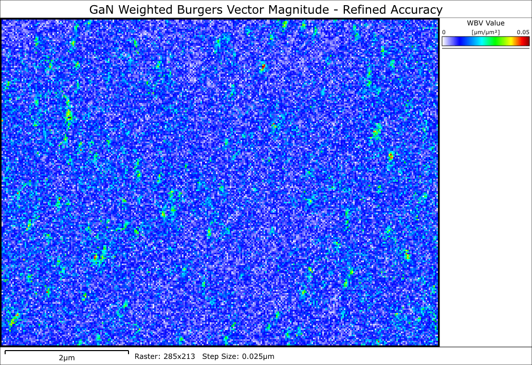
Standard indexing of EBSD patterns using the Hough-transform will typically have an orientation precision of 0.1-0.5°. The use of advanced indexing methods, such as Refined Accuracy, can improve the precision to <0.05°.
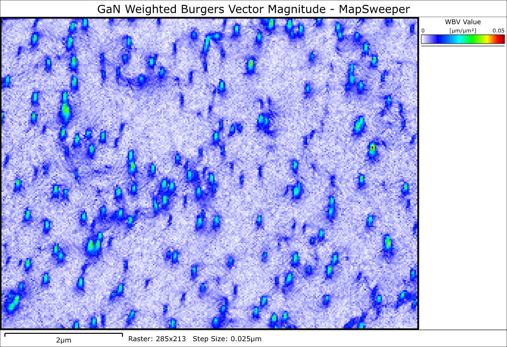
However, with hybrid pattern matching techniques, it is possible to further improve the precision to ~0.01° or better. This has multiple benefits, but primarily it helps with the analysis and interpretation of small orientation changes such as resulting from the formation of dislocation structures in materials (either as-grown or due to deformation).
In MapSweeper, the refinement process is fast and simple, and follows these steps:
This process will typically involve the generation and matching of 100-200 simulated EBSD patterns and, depending on the computing power and the EBSD pattern resolution, can take less than 1 ms. The final orientation precision will depend on the quality of the EBSD patterns; however, even for relatively low resolution or noisy EBSD patterns, the orientation refinement process can deliver significant improvements when compared to Hough-based indexing.
Screen capture showing the progressive refinement of the orientation of an EBSD pattern from a ferritic steel. Left – experimental EBSP. Right – Dynamical simulations showing the orientation optimisation. The normalised cross correlation coefficient increased from R=0.72 to R=0.79 during this optimisation.
Here we have introduced the concept of pseudosymmetry and outlined ways to prevent misindexing or to filter out systematic errors. However, there is a limit to the resolution of such approaches – in the example provided previously (gamma TiAl), the difference between the c and a lengths of the unit cell are ~1.8%. For smaller c:a ratios, these conventional approaches may not work effectively.
In such cases a hybrid pattern matching approach can work well and, with sufficient EBSP quality, will resolve pseudosymmetry effects down to <0.5% unit cell difference. The method used by MapSweeper is very simple:
The pseudosymmetry correction method is also combined with an orientation refinement approach to ensure that the optimised orientation is calculated for each pseudosymmetric solution. The resolution of this method is very dependent on the quality of EBSD patterns and the corresponding R value. For good, noise free EBSD patterns, R values > 0.7 enable the resolution of unit cell variations below 0.5%, but for noisier patterns (and smaller R values), greater unit cell differences will be required to ensure robust results. The simulated patterns from a CuInSe2 structure (tetragonal, but ~0.5% from cubic) illustrate the subtle changes that can be picked out by MapSweeper.
Dynamical simulations showing 2 (90° rotated) orientations of CuInSe2, highlighting the subtle pattern changes associated with the pseudosymmetry.
Some crystal structures are non-centrosymmetric (i.e. they lack an inversion centre). In some cases, this lack of an inversion symmetry corresponds to important properties of the material, such as the piezoelectric effect. The point groups that lack inversion symmetry can be polar or chiral, and the polarity or chirality of the structure has a small but measurable effect on the EBSD pattern.
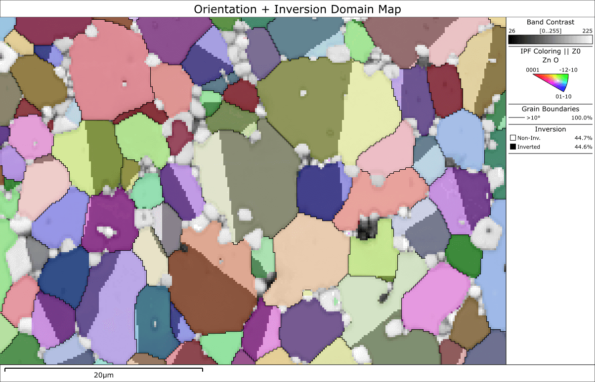
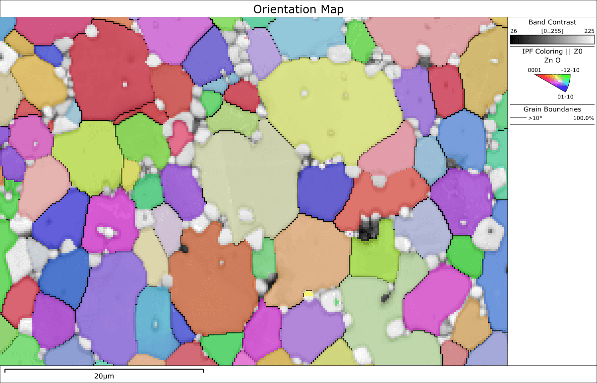
This change in pattern is much too subtle to be measured using standard (Hough-based) indexing methods but can be detected using the hybrid pattern matching approach within MapSweeper. The methodology is very similar to that used to resolve pseudosymmetry outlined above, with the pattern matching process being applied to the inverted structure as well as the non-inverted structure. Likewise, good quality EBSPs are required in order to effectively resolve the polarity or chirality of materials, as shown in the example below from a ZnO grain.
Animation (from the MapSweeper interface) showing the effect of inversion on the normalised cross correlation coefficient for a ZnO EBSD pattern. Left – experimental pattern. Centre – simulated pattern, switching from a non-inverted to an inverted structure. Right – difference between the experimental and simulated patterns. Note the higher R value associated with the inverted structure.
In materials that contain several phases with very similar crystal structures, conventional EBSD can struggle to differentiate between the correct and incorrect solutions. Here we have introduced alternative approaches to separating phases, such as the use of elemental information from EDS, or the width of Kikuchi bands in the pattern.
However, MapSweeper incorporates a hybrid pattern matching approach that enables a more robust phase discrimination, even between phases that are very close in structure.
The approach taken in MapSweeper is as follows:
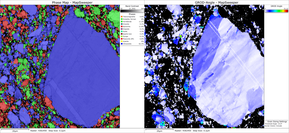
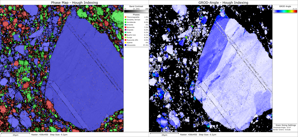
This approach will slow down the analysis, as any point indexed as one of the grouped phases needs to be “swept” using all phases in the group, but the method is very effective at separating phases, even using low resolution or relatively noisy EBSD patterns. The results can be seen in the adjacent video, illustrating how the phase separation works together with the orientation refinement process to enhance a dataset from a deformed Ni superalloy sample.
Video showing MapSweeper Refinement of a dataset containing a small cubic Ti2CN precipitate in a Ni superalloy. The 2 phases have been grouped together using MapSweeper, ensuring robust phase separation that was not possible using conventional Hough-based indexing, as well as improved orientation precision.
Here we describe how hybrid pattern matching is used in AZtecCrystal MapSweeper to repair existing EBSD datasets. In a Repair Sweep, MapSweeper can fix indexing errors from the original analysis, and iteratively index pixels that were not solved originally. The repair sweep typically works together with the Refinement sweep (and it uses the pattern and simulation resolution defined in the Refinement sweep step), but it can also be used on its own (for example on datasets where only the non-indexed EBSPs were saved).
There are 2 operations that can be selected in the Repair sweep, as explained below.
Hough-based indexing rarely indexes 100% of the points in a dataset. Typically, overlapping patterns collected at grain boundaries can result in non-indexing (as insufficient Kikuchi bands match the structures from either orientation), as well as in areas / grains where the EBSD pattern quality was too poor for reliable band detection using the Hough transform. This is commonly the case in highly deformed samples and in nanocrystalline materials (such as analysed using transmission Kikuchi diffraction (TKD)).
The Repair sweep in MapSweeper solves non-indexed points by utilising the orientation and phase information from adjacent, indexed points as follows:
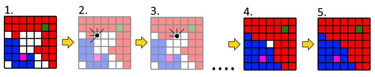
Note that this is not a duplication of the adjacent measurements, but the algorithm uses those adjacent measurements only as a starting point for the initial simulated EBSP. Solutions are only accepted if they result in a sufficiently high R value following refinement, ensuring that false indexing does not occur.
This hybrid method of “reindexing” the zero solution pixels is much faster than using a full “brute force” indexing method (such as DTM, or Dictionary / Spherical indexing) and produces very comparable final results with a high degree of angular precision. The only requirement is that the initial indexing rate is sufficiently high to avoid large areas of non-indexed pixels (such as whole grains).
Sometimes individual EBSD patterns, or the patterns from clusters of a few adjacent points, are incorrectly indexed during Hough-based indexing. This can be due to a locally poor quality pattern, or due to certain crystallographic properties of the phases present in a sample. Usually such “wild spikes” or small clusters are removed from a dataset during a post-analysis clean up and are replaced by duplications of one of the adjacent measurements.
During the Repair Sweep in MapSweeper, these isolated clusters (up to 5 pixels in size) are matched with simulations derived from their initial measurement (which may be incorrect) as well as from the adjacent measurements, as follows:
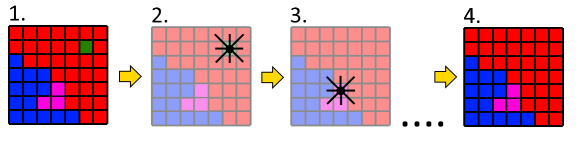
The combination of the removal (or verification) of cluster pixels, plus the reindexing of initially non-indexed patterns, makes the Repair Sweep a very effective tool for enhancing EBSD datasets. The process is both fast and results in fully refined orientation data for each measurement point. The following example shows how the use of a Refine Sweep followed by a Repair Sweep produces essentially identical information as when using the DTM indexing method, but in a fraction of the time.
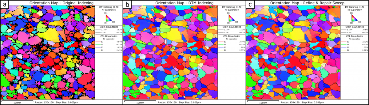
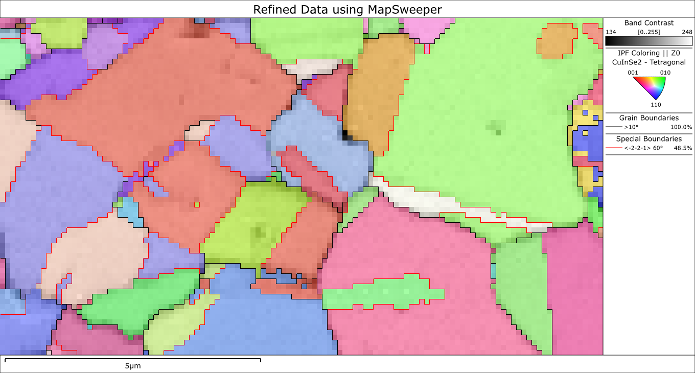
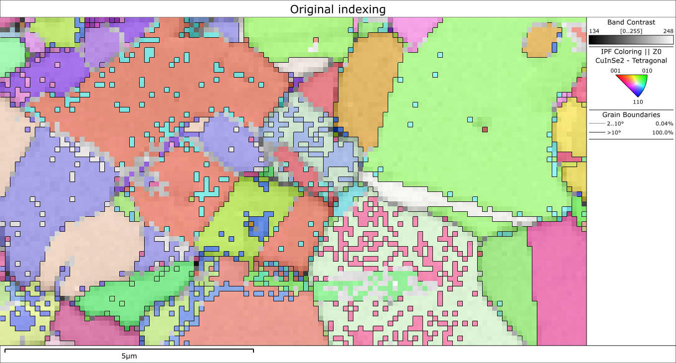
Example TKD dataset from a nanocrystalline Ni sample, showing the benefits of the MapSweeper Repair sweep. (a) Original Hough-based indexing (80% indexing). (b) Results of reindexing using the Dynamic Template Matching method (99.9% indexing, 13 minute reanalysis). (c) Results following a Refine Sweep followed by a 2-pass Repair Sweep (99.9% indexing, 90 second reanalysis).
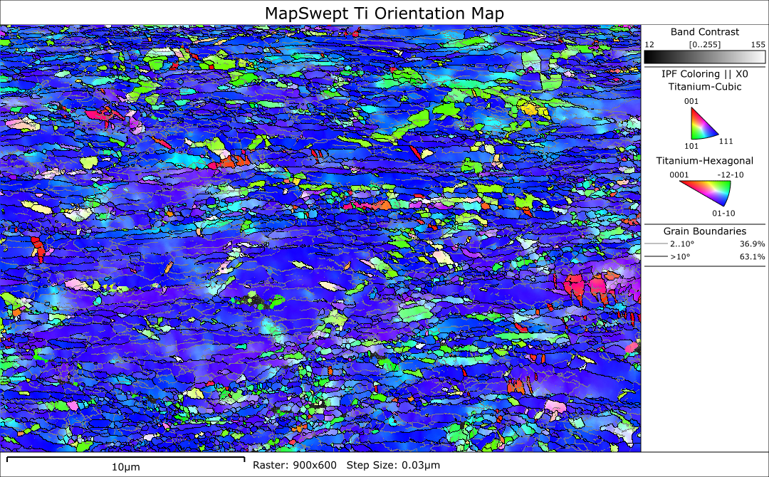
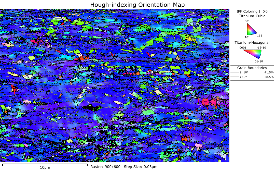
Here there are a number of examples showing how the different Sweep modes in AZtecCrystal MapSweeper can be used to enhance many different types of EBSD and TKD datasets. In each case, use the slider to change the display from the original data (as collected using conventional Hough-based indexing) to the MapSwept data.
© Oxford Instruments 2026