
EBSD Explained
Techniques
Applications
Hints and Tips
Technology
OXFORD INSTRUMENTS EBSD PRODUCTS
CMOS Detector RangeAZtecHKL Acquisition SoftwareAZtecCrystal Processing Software
The analysis of the dislocations in a material can provide a lot of useful information about the characteristics of deformation and strain, as well as about growth defects in single crystals. Every dislocation within the crystal lattice causes a very small change in orientation, due to the shift in the rows of atoms; although this orientation change is usually too small to be measured accurately using EBSD, the accumulated orientation change (or the curvature of the lattice) caused by many dislocations of the same sign can be measured. This is schematically illustrated in the following image, showing how dislocations of the same “sign” can contribute to significant lattice curvature, whereas mixed signs of dislocations may not cause any net lattice curvature at all.
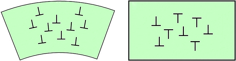
Schematic illustration showing (left) how dislocations of the same sign will contribute to a significant bending of the crystal lattice (i.e. plastic deformation), whereas dislocations of mixed signs (right) will cancel each other out and not result in any significant lattice bending.
All materials contain dislocations with mixed signs, and these are sometimes referred to as statistically stored dislocations (SSDs). Those dislocations of the same sign that contribute to a net lattice curvature are usually referred to as geometrically necessary dislocations (GNDs) and these are what, in most cases, we can use the EBSD technique to measure.
The fact that the lattice curvature caused by GNDs is measurable by EBSD means that it is possible to extract significant details about the GND densities and types using EBSD, and there have been many research papers on this topic in recent years.
The fundamentals of dislocation characterisation are given in a seminal publication by Nye (J.F. Nye, Some geometrical relations in dislocated crystals, Acta Mater. 1 (1953) 153–162) in which the relationship between lattice curvature and dislocation density was presented. Many subsequent papers have explored different approaches to determining the GND densities using orientation data collected by EBSD, such as the following examples:
In AZtecCrystal, a licensed viewing mode enables advanced dislocation analysis using an approach known as the “Weighted Burgers Vector” (WBV) technique. This technique is based on work published by Wheeler et al. in the following paper:
The principles of the technique are once again based on those of Nye (1953), and the Weighted Burgers Vector is defined as:
W = sum, over all types of dislocations, of [(density of intersections of dislocation lines with map) × (Burgers vector)]
The results are “weighted” because of the 2D nature of the EBSD dataset. Dislocation lines that intersect the map area at a high angle will be more likely to be measured than dislocation lines that are at a shallow angle to the mapped surface. Those dislocation lines that are parallel to the sample surface will not contribute to the measurement at all. Therefore, the dislocation densities that are calculated will always be a minimum limit of the true dislocation density (i.e. the true dislocation density in the sample will almost always exceed that measured using 2D EBSD). Despite this minor limitation, the WBV approach provides significant insights into the dislocation types and densities within crystalline materials and is free of a number of the assumptions that are necessary in other dislocation analysis methods. Indeed, the only assumption made in the WBV method is that elastic strains are small, so that the lattice distortion is entirely due to dislocations.
The standard way to calculate the WBV is via a “differential” approach, in the same way as used in many other methods (and using the same pixel array approach as for kernel average misorientation – KAM - maps); i.e. calculating the local orientation gradient at each point and determining the necessary dislocation content to account for that gradient. However, AZtecCrystal utilises the “integral loop” approach proposed by Wheeler et al.; in effect a series of “Burgers circuits” are plotted on the map surface. Normally the Burgers circuits are applied in crystallographic coordinates (e.g. for measuring the Burgers vector by tracing the atom positions around a single dislocation), but the Burgers circuit can also be applied on the sample surface. This is a closed loop, with each small change in orientation around the perimeter of the loop attributable to a small component of the total net Burgers vector. The comparison between Burgers circuits in crystallographic and sample coordinates is elegantly represented by the following image:
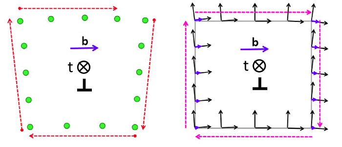
Figure showing “Burgers circuits” in crystal (left) and sample (right) reference frames. Note how they both give the same Burgers vector (central purple arrow, b): in the case of the sample reference frame the loop is closed, so b is the net sum of the individual vectors at each step (small purple arrows). For the loop in Crystal coordinates, the Burgers vector is the incomplete section of the circuit. Image modified from Konijnenberg et al. (2015).
In AZtecCrystal, a Burgers circuit is traced around each point in the map (with user-defined size and shape), and the weighted Burgers vector is calculated for each point. This sliding loop dislocation analysis is less susceptible to the noise in the orientation measurements and will therefore provide a more accurate determination of the local Burgers vector magnitude and the Burgers vector orientation. However, a downside of the sliding integral loop approach is that if the loop perimeter crosses a 2nd phase or a high angle boundary, then no result is returned. This will mean that there will be no data in the points immediately adjacent to high angle or phase boundaries.
The improved noise level of the sliding loop WBV approach compared to a conventional differential approach is clearly shown in the following images. These are taken from a GaN thin film that contains individual threading dislocations. With the additional angular precision achieved when indexing using the Refined Accuracy method, the small changes in orientation about each dislocation (< 0.1°) can be detected and the nature of these dislocations effectively studied using the WBV approach. The reduced noise in the WBV sliding loop map compared to the KAM map is clear, and correlation with an electron channelling contrast image (ECCI) of the same area shows that the dislocations are being reliably picked out.


Images from a GaN thin film with threading dislocations. Left – Kernel Average Misorientation (KAM) map collected using a 5x5 pixel array. Centre – Sliding loop WBV map using a 5x5 pixel loop size. Right – Electron channelling contrast image showing the individual dislocations. Note the far lower noise levels in the WBV map that enables reliable analysis of the individual dislocations.
The output of the WBV approach is 3 fold:
All 3 of these outputs can provide important information about the nature and distribution of dislocations in a sample and help researchers to understand the mechanisms of deformation in a material.
In this example, 2 Ti-alloys were deformed under different conditions (strain rate / strain / temperature) and the microstructures analysed using EBSD to characterise the mechanisms of deformation.
The dislocation density maps of the 2 samples are shown below: there are minor differences between the GND densities which are more easily quantified when the full distribution of GND density values are plotted.
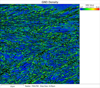
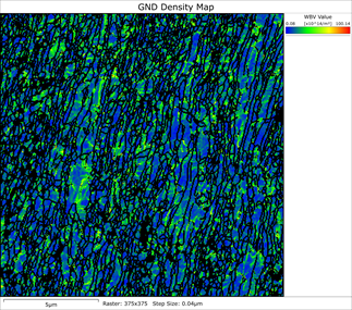
Geometrically necessary dislocation density maps calculated using the WBV technique. Sample 1 (load direction || X), sample 2 (load direction || Y). Note the slightly higher maximum GND density for sample 2 (1 x 10¹⁶ m-2 compared to 7.6 x 10¹⁵ m-2)
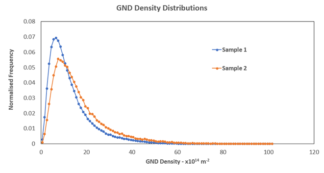
GND density distributions for the 2 Ti samples. The mean GND values for the 2 datasets are 1.25 x 10¹⁵ m-2 for sample 1, 1.62 x 10¹⁵ m-2 for sample 2.
However, the most significant difference between the 2 datasets is in the orientations of the weighted Burgers vectors. For sample 1, the WBV orientations show a strong clustering on the basal plane, close to the <a> direction, which is consistent with dominant slip on the <11-20>(0001) slip system. In contrast, the second sample shows WBV orientations weakly clustered closer to the <c> axis: this would be consistent with significant activation of non-basal slip, such as pyramidal slip with <c+a> Burgers vectors.


Weighted Burgers vector orientations in crystallographic coordinates for sample 1 (left) and sample 2 (right). The plots only show the WBV orientations for WBV magnitudes >15 % of the maximum WBV value for each dataset.
Further examination of the boundary planes, associated boundary rotation axes and the texture of the samples helps to further characterise the nature of the slip systems in these samples. However, from the results presented here, we can see that a simple comparison between the GND densities of the 2 samples is insufficient to identify significant differences between their respective deformation styles, whereas a study of the Burgers vector orientations quickly highlights very contrasting styles of slip.
© Oxford Instruments 2026